On the Collapsing of Manifolds with Local Rewinding Reifenberg Control
Shaosai Huang
∗ Working paper. Comments welcome.
Kspectra Research Inc., Toronto, Canada
Abstract
Let be a complete Riemannian manifold with whose local universal covers are uniformly -Reifenberg-close to below a fixed radius . We show that for every there are and such that, if , a complete Ricci flow with exists on and satisfies for . On closed manifolds this is a uniform lower bound for the lifetime of the Ricci flow; on noncompact manifolds, where the initial curvature may be unbounded, it is an existence theorem, and the flow is unique among complete Ricci flows from with a curvature bound of the form . The key step is a localized comparison of two Ricci flows through the Ricci–harmonic map heat flow, following Lee, which transfers a Type-I curvature bound from a complete comparison flow to the incomplete flow lifted to a local cover. Consequently, below a dimensional Reifenberg threshold, collapsing closed manifolds admit singular nilpotent fibrations over their Gromov–Hausdorff limits. Conditional on Nifa’s construction, the Reifenberg hypothesis cannot be weakened to noncollapsing of the local covers: products of shrinking circles with Nifa’s four-manifolds have and uniformly noncollapsed local covers, but admit no continuous Gromov–Hausdorff approximations with small error onto their limit.
The model is collapse under a two-sided sectional-curvature bound. If closed -manifolds with collapse
to a compact metric space , Fukaya and Cheeger–Fukaya–Gromov [Fuk87; Fuk89; CFG92] construct
-equivariant nilmanifold bundles on the frame bundles, and passing to -orbit spaces gives continuous
maps with infranilmanifold fibres. Following [Ron26b, Section 1.3], a singular nilpotent fibration is a
quotient map arising in this way; the full diagram, with its metric and differential estimates, is
recalled in Theorem 8.1.
We ask how much of this survives under a Ricci lower bound alone. A metric ball may then itself
be collapsed, so the local hypotheses are imposed on its Riemannian universal cover. We compare two
such conditions.
Definition 1.1 (Local Rewinding Conditions). Let be a Riemannian manifold, and , and let
be the Riemannian universal cover of the open ball. The point is a -local rewinding
Reifenberg point, abbreviated -LRRP, if
for the pointed Gromov–Hausdorff distance, the
centres of the balls being the base points. The manifold has uniform -LRRP if every
point is a -LRRP. The point is a -local rewinding volume point, abbreviated -LRVP, if
The terminology follows [HRW20; Ron26a; Ron26b]. LRRP controls the balls about in the local
cover at every scale below , LRVP only the volume of the ball of radius . Under , LRRP with implies
LRVP with by Colding’s volume convergence theorem [Col97]; the converse fails. Rong’s conjecture
under the stronger condition reads as follows.
Conjecture ([Ron26b, Conjecture 0.6, case (0.6.1)]).Let be closed -manifolds. Assume that
and that all their points are -LRRP points. Suppose that converges in the Gromov–Hausdorff
topology to a compact metric space of positive diameter and that . Then, for large, there is a
singular nilpotent fibration .
Rong uses the unpointed distance in (1.1), which changes by at most a factor of two
(Section 2.1). Rong’s definition requires ; we prove the conjecture for and show that the conclusion
fails in general for .
Under the weaker LRVP hypothesis the picture is different. The earlier proposals under a Ricci
lower bound and uniform LRVP all expect, at a minimum, that the convergence is realized by
continuous maps whose approximation errors tend to zero. Case (0.6.2) of Conjecture 0.6 in
[Ron26a] asks in addition for finite infranil-quotient fibres capturing the short loops. Open
Problem 4.4 of [Ron26b] fixes , writes for the -regular region and puts
A smooth infranil bundle
is already available over , and the problem asks whether it is the restriction of such a
map. Our examples show that under LRVP the continuous approximation itself need
not exist, so both statements fail regardless of their requirements on the fibres or over
.
1.1Main Results
Uniform LRRP supplies what ordinary short-time existence on a closed manifold lacks: control
independent of the initial curvature.
Theorem 1.2 (Uniform Lifetime on Closed Manifolds).Fix , and . There are and with the
following property. If is closed, , and every point of is a -LRRP, then the maximal Ricci flow with satisfies
The second result allows complete noncompact data with unbounded initial curvature.
Theorem 1.3 (Complete Manifolds).Fix , and . There are constants and , depending only
on and , respectively, with the following property. If is complete, , and every point of is a -LRRP, then there is a complete Ricci flow , smooth on , with and
It is the only
complete Ricci flow on with initial metric whose curvature satisfies for some constant
.
For noncompact the existence is new; the uniqueness recovers [Lee26, Theorem 1.1] by the
same comparison argument. At positive time, Theorem 1.2 gives a bounded-curvature
metric uniformly bi-Hölder to , so bounded-curvature collapsing theory applies. For a map
between metric spaces put
is an -Gromov–Hausdorff approximation if and is -dense in
.
Theorem 1.4 (Singular Nilpotent Fibrations).For every there is with the following property. Let
, and let be closed -manifolds with and uniform -LRRP. Suppose that they converge in the
Gromov–Hausdorff topology to a compact metric space of positive diameter, and that . Then there
are and, for large, continuous surjective maps such that
(i)
is an -Gromov–Hausdorff approximation from to ;
(ii)
every fibre of is an infranilmanifold of positive dimension;
(iii)
is a singular nilpotent fibration: it is induced by an -equivariant fibre bundle, with nilmanifold fibre and affine structure group, from the frame bundle of onto a closed manifold with homeomorphic to .
This is case (0.6.1) of [Ron26b, Conjecture 0.6] for , in the precise form of Theorem 8.2 and
with the qualification in Section 1.4. If the are moreover aspherical with fundamental
groups of type , Corollary 8.4 shows that is homeomorphic to, and hence abstractly
smoothable as, an aspherical manifold: the manifold and asphericity part of [Ron26b,
Conjecture 0.7], without its quantitative Reifenberg conclusion for the original metric on
.
Under the weaker condition, Nifa’s closed four-manifolds [Nif26] give limits onto which there are
no continuous almost-isometries.
Theorem 1.5 (No Continuous Approximation).Let be the closed four-manifolds of [Nif26,
Theorem 1.3], and let be their Gromov–Hausdorff limit. Let with , and give the product metric.
Then the following hold.
(i)
, and there is such that every point of every is a -LRVP.
(ii)
in the Gromov–Hausdorff topology, , and .
(iii)
There are and such that for every continuous map with . In particular, for and there is no continuous -Gromov–Hausdorff approximation from to .
(iv)
is not locally contractible, and it is not homeomorphic to the orbit space of a smooth action of a compact Lie group on a manifold.
(v)
Every point of every is a -LRRP for all and all , while for no and no do all the have uniform -LRRP.
Part (iii) excludes every conjectured structure, each of which includes continuous
Gromov–Hausdorff approximations with errors tending to zero.
Corollary 1.6 (The Statements under LRVP).The manifolds of Theorem 1.5are closed
five-manifolds with and uniform -LRVP that collapse to the compact space . For this sequence:
(a) there is no singular nilpotent fibration for large, so Theorem 1.4fails with LRRP replaced
by LRVP, or by -LRRP with ; (b) case (0.6.2) of [Ron26a, Conjecture 0.6] fails; (c) [Ron26b,
Open Problem 4.4] has a negative answer; and (d) [HRW20, Conjecture 3.3] fails whenever
a singular fibration is, in particular, a continuous Gromov–Hausdorff approximation onto the
limit with error tending to zero.
The Reifenberg constant of a sequence is the infimum of the for which some gives uniform
-LRRP. For it lies between and ; the upper bound holds for every product of a circle with a
complete four-manifold of nonnegative Ricci curvature.
1.2Mechanism and Proof Strategy
Theorems 1.2 and 1.3 rest on a local statement for a Ricci flow that need not be complete,
Proposition 3.1: an curvature bound on the initial ball , with a Ricci lower bound and Euclidean
closeness on at time zero, improves at to , , for a time proportional to . Applied with on each local
cover, a first-time argument gives the uniform lifetime (Section 3).
For the local statement, Reifenberg control and the initial Ricci bound give almost-Euclidean
isoperimetry [Col97; CM20]; Hochard’s conformal completion [Hoc16; HW22] produces a
complete metric that agrees with the original one on a smaller ball, and its Ricci flow has a
bound with by Wang’s pseudolocality theorem [Wan20] (Section 4). A localized version
of Lee’s comparison through the Ricci–harmonic map heat flow [Lee26] transfers this
bound to the incomplete lifted flow (Sections 5 and 6). The Ricci lower bound enters only at time zero, only the comparison flow is complete, and distinct local covers are never
compared; the inequality between the conformal and original metrics replaces the one global
distance-conversion step in Lee’s argument and avoids the patching issue noted in [Ron26b,
Section 1.3].
For noncompact data, conformal metrics equal to on an exhaustion push the artificial boundaries
to infinity; isoperimetry on the local covers survives at an adaptive scale near the collar, and local
estimates through time zero [Che09; ST21] give a complete limit flow (Section 7). For Theorem 1.4,
the distance distortion estimate of [HW22, Appendix A] identifies the smoothed and original limits
bi-Hölderly, and the theory of Fukaya and Cheeger–Fukaya–Gromov supplies the fibrations
(Section 8).
Theorem 1.5 (Section 9) is independent of the Ricci flow. The circle factor gives the
rewinding-volume bound; a small-distortion map would have degree one over the regular part of and
so wrap around infinitely many copies of minus a ball, which would give infinitely many
independent classes in the finite-dimensional space ; the Reifenberg bounds follow from
Bishop–Gromov and, at the accumulation point, from the conical tangent via the quantitative
Borsuk–Ulam theorem [DS81; LMS23].
1.3Relation to Prior Work
The nilpotent structure under bounded sectional curvature is due to Fukaya [Fuk87; Fuk89] and
Cheeger–Fukaya–Gromov [CFG92]; the programme under a Ricci lower bound is surveyed in
[HRW20]. For manifold limits, Rong obtained affine nilpotent bundles without smoothing [Ron26a,
Theorem B], [Ron26b, Theorem 0.12], and Huang and Wang [HW22] used uniform Ricci-flow
smoothing under Euclidean or flat-orbifold models with a maximal-rank hypothesis. Theorem 1.2
imposes no condition on the collapsed limit.
Our analytic tools originate in Hochard’s conformal completion [Hoc16], the complete-flow
limit of Simon–Topping [ST21], Lee’s comparison and uniqueness theory [Lee26], and
Wang’s scale-invariant refinement [Wan20] of Perelman’s pseudolocality theorem [Per02,
Theorem 10.1]; the entropy input follows from scalar-curvature and isoperimetric bounds [Wan18,
Lemma 3.5].
Under LRVP, Rong’s six-dimensional example already excludes a singular nilpotent fibration but
still admits continuous approximations [Ron26b, Example 4.2]; see Section 10.2. Our examples
exclude even those.
1.4Scope and Organization
Theorems 1.2 to 1.4 rest on the Ricci–harmonic map method of [Lee26] and the pseudolocality
theorem [Wan20, Theorem 1.2]. The local estimates we need are collected in Proposition 2.3; its
part (iv) is proved in Section 2.4 from [Lee26, Lemma 2.5] and the local maximum principle of
[LT22], and its other parts in Appendix A, using the short-time existence lemma of [BK22]. The
localized comparison is proved in Section 5, and complete Type-I uniqueness is derived in Section 7.
Corollary 8.4 also uses [Ron26b, Theorem A]. Theorem 1.5 and Corollary 1.6 are independent of the Ricci-flow results and conditional on the unrefereed construction [Nif26], whose required
properties are listed in Section 9.1.
The constants , and are small and not computed. In Theorem 1.4 the frame-bundle diagram is
formed with the metrics smoothed by Ricci flow, since a Ricci lower bound does not control the
canonical frame-bundle metric; the identification is therefore bi-Hölder rather than isometric,
although the are Gromov–Hausdorff approximations for the original metrics. We prove
neither the quantitative Reifenberg regularity of the original limit metric in [Ron26b,
Conjecture 0.7] nor case (0.6.2) of [Ron26b, Conjecture 0.6]; Section 10 discusses the remaining
cases.
After the preliminaries, Sections 3 to 6 prove Theorem 1.2; the remaining principal results are
proved in Sections 7 to 9.
2Preliminaries
We fix metric conventions, the local completeness available on local universal covers, and the analytic
inputs of Wang and Lee.
2.1Conventions
Manifolds are smooth and connected, and “closed” means compact without boundary. Write and for
Riemannian balls and distance, and in a metric space. A regular domain is relatively compact, open,
and smoothly bounded; is the volume of the Euclidean unit ball. Ricci flows satisfy . Constants
display their dependencies when needed; unadorned depend only on the parameters of the current
statement and may change by line.
A correspondence between metric spaces and is a subset whose two projections are onto, and its
distortion is
The Gromov–Hausdorff distance is [BBI01, Theorem 7.3.25]. For pointed spaces we use
This is at least the unpointed distance. For balls with displayed centres, including (1.1) and (3.3),
is pointed. If every point of lies within of and a correspondence between and has
distortion at most , every point related to has norm at most ; adding therefore at most
doubles the distortion. Thus Rong’s unpointed form of (1.1) implies ours with in place of
.
2.2Local Universal Covers
The local covers are incomplete. For call its depth. Positive depth supplies the following local
substitute for completeness.
Lemma 2.1 (Local Completeness of the Cover).Let be a complete Riemannian manifold, and ,
and let have depth .
(i)
The exponential map of at is defined on the open ball of radius in the tangent space.
(ii)
For , the closed ball of radius about is compact, and each of its points is joined to by a minimizing geodesic.
(iii)
If and , then .
Proof.For , . Thus every -geodesic from of length below stays in and lifts, proving (i). The
local Hopf–Rinow proof [Car92, Chapter 7, Theorem 2.8] gives (ii), and the standard Jacobian
comparison along these minimizing geodesics gives (iii).∎
2.3Local Entropy and Pseudolocality
For a metric on an -manifold, a relatively compact ball and , the local entropy of [Wan18] is the
infimum of
over and with and . Wang’s pseudolocality theorem turns a lower bound for this
entropy into a scale-invariant curvature bound; Section 4 uses it to give the comparison flow its
Type-I bound.
Theorem 2.2 (Wang’s Pseudolocality Theorem [Wan20, Theorem 1.2]).For every positive smaller than there is with the following property. Let , , be a complete Ricci flow with bounded
curvature on an -manifold, and let be a point of the manifold. If
then on for every
.
2.4Ricci–Harmonic Comparison Inputs
We use the Ricci–harmonic gauge method of [Lee26, Sections 2–3]. The following proposition states
the local versions needed here; Appendix A supplies the existence and derivative proofs. Derivatives
of a solution use and ; when is a diffeomorphism onto its image, is Ricci–DeTurck relative to
.
Proposition 2.3 (Local Comparison Estimates).All source and target manifolds have dimension
. Let be a threshold below which the discrepancy inequality (2.1) below holds, and set
.
(i)
Local Existence. For every there is with the following property. Let be a smooth domain, let a possibly incomplete Ricci flow be smooth on a neighbourhood of , let carry a complete Ricci flow , and suppose, on , that for some
while all curvature derivatives of are globally bounded on . If is smooth on a neighbourhood of and , then the Ricci–harmonic map heat flow starting from exists, with , on
Ricci–DeTurck Decay. Given and an integer there is a constant , depending only on , , and , with the following property. Let be a smooth Ricci flow on with and there, and let be a smooth Ricci–DeTurck flow relative to on a neighbourhood of the closed reference cylinder , with , satisfying there
Then, on and for ,
Proof of part (iv). Rescale and write
so that on by hypothesis. The covariant discrepancy
equation gives, for small ,
see [Lee26, Lemma 2.5]; there the term absorbs the quadratic gradient
terms, and replacing the operator of by costs . Both flows are smooth on the closed cylinder, so is
bounded there; only the bound degenerates at . After enlarging , one also has and for . For each ,
the ball of radius about has closure in . Since , [LT22, Theorem 1.1], with an integer
exponent , therefore gives uniformly
for any prescribed integer , on a time depending only on
.
For , the shrinking-balls lemma [ST21, Lemma 2.2], applied to , gives for a common smaller
time. Along a unit-speed -geodesic of length , which exists because is relatively compact, express in
a parallel frame and apply Taylor’s formula to each component. This gives
Choose and decrease
the time to absorb the spare factor of in the square of (2.2). Restoring gives the two
bounds.∎
Section 5 applies these estimates on successive time slabs.
3The Local Improvement and the First-Time Argument
We state the local improvement for incomplete flows and derive Theorem 1.2; Sections 4 to 6 prove
the local statement.
Proposition 3.1 (Local Type-I Improvement).Fix , and . There are , , and with the
following property. Let , , be a smooth Ricci flow on an -manifold , let and , and assume
that
(a)
the closed ball is compact;
(b)
on ,
(c)
on ,
(d)
Then
and consequently
All hypotheses concern the initial ball, because no Ricci lower bound is assumed at positive time.
Lifting the global flow to each local cover and applying the gain while gives the following first-time
argument.
Proof of Theorem 1.2. Apply Proposition 3.1 with and the prescribed . Let be its constants and
put
Hamilton’s theorem [Ham82] starts the maximal flow for a positive, possibly nonuniform
time.
Fix and lift the flow to the fixed -cover . Since , Lemma 2.1 makes the closed -ball
about compact, while (1.1) gives
The choice and the initial Ricci lower bound give
Define
Smoothness gives . Before , every lifted flow satisfies Proposition 3.1 with and , hence
If
and , the strict margin and continuity extend (3.6); if , (3.7) bounds curvature on the final
half-interval and continuation extends the flow. Thus
One final application at every lifted point gives
(1.2) with .∎
4A Complete Comparison Flow
We construct the complete comparison flow using Hochard’s conformal completion [Hoc16; HW22]
and Theorem 2.2. The rescaling-invariant lemmas are stated for reuse in Section 7.
4.1Constants
Set . This is the Type-I constant of the comparison flow: it lies below Wang’s threshold , and its gap
to absorbs the comparison error in (6.2). Let be from Theorem 2.2, and put and ; in Lemma 4.3
the isoperimetric deficit gives the entropy bound of Theorem 2.2, and fixes the lifetime of the
comparison flow relative to the isoperimetric scale. Choose the parameter of the conformal profile of
Lemma 4.2 and then the isoperimetric deficit of the initial metric so that
All these constants
depend only on and .
4.2Initial Isoperimetry
The first lemma converts the initial hypotheses into definite-scale isoperimetry.
Lemma 4.1 (Initial Isoperimetry).For every there are constants , and , depending only on and ,
with the following property. Let be a Riemannian metric on an -manifold, let be a point and , and
suppose that the closed ball of radius about is compact and that
Then, with ,
and every regular
domain satisfies
Proof.Scale to . Let be the constants of [CM20, Theorem 1.1] for lower Ricci bound and dimension
. Choose , , and so that
We use Colding’s local volume continuity [Col97, Main Lemma 2.1 and
Theorem 0.1] in the following form. There are and such that on and imply ; this is the form used
in [HW22, proof of Lemma 2.4].
Set and . Restricting a correspondence in (4.2) to concentric balls and rescaling gives
where
with . These balls correspond to relatively compact -balls in . Choose so that this error is below , ,
and . Thus , and [CM20, Theorem 1.1] gives, for finite-perimeter ,
The parameter choice, the
th power, and rescaling prove (4.4) with . Finally (4.2) gives ; decreasing until proves
(4.3).∎
For , fix
the constants of Proposition 3.1, all depending only on .
4.3Conformal Completion
The next conformal change is supported outside a smaller ball and nearly preserves isoperimetry; its
domain is a superlevel-set component of the cutoff.
Lemma 4.2 (Conformal Completion).For every there are constants and , depending only on , and , with the following property. Let be a Riemannian metric on an -manifold, let be a point and ,
and suppose that the closed ball of radius about is compact, that (4.3) holds, that (4.4) holds with ,
and that there is a smooth function with values in , supported in and equal to one on , such that
Then there are an open set with
and a smooth function on such that has the following properties,
where :
(i)
is complete, , and on ;
(ii)
has bounded curvature;
(iii)
;
(iv)
every regular domain compactly contained in an -ball of radius satisfies
Proof.Choose a regular value of and let be the component of containing ; it has smooth compact
closure in . Fix a smooth decreasing with near , , , and for , and set
where . The smooth extensions of past have finite curvature and Hessian norms
there.
Let be Hochard’s conformal profile [Hoc16, proof of Lemma 6.2], smoothed as in [HW22,
equations (2.3)–(2.5)]: it is nondecreasing and convex, vanishes on , tends to infinity at , and satisfies
For and , it also satisfies
Set and . The second estimate in (4.10) and (4.8) make every escaping
curve have infinite -length. Thus is complete, dominates , and equals on . The conformal
scalar-curvature formula, (4.3), (4.8), and (4.9) give
The full-curvature formula and the finite bounds
on give bounded sectional curvature.
Call the set , where , the collar. For a point of the collar put and . The calculation
of [HW22, equations (2.23)–(2.33)], or the same first-exit argument using (4.8)–(4.10),
gives, for ,
where the metric inequality holds on the displayed ball, which lies in in the
original metric. Comparing boundary area and volume with the two conformal factors, (4.4)
and (4.10) give, for every regular domain compactly contained in that ball,
The middle
inequality is (4.1). Set . Then (iii) holds. An -ball contained in satisfies (4.4); otherwise it
meets the collar and lies in a -ball to which (4.11) applies. Domain monotonicity proves
(iv).∎
The curvature bound in (ii) is qualitative; the next lemma uses it only to start the Ricci flow of
.
Lemma 4.3 (Complete Comparison Flow).Let be a complete Riemannian metric with bounded
curvature on an -manifold , and let . Suppose that and that every regular domain compactly
contained in an -ball of radius satisfies (4.7). Then has a complete bounded-curvature Ricci flow on
, and
Proof.Shi [Shi89] starts a complete bounded-curvature flow. Let precede its maximal time. At each ,
the scalar and isoperimetric hypotheses and [Wan18, Lemma 3.5] give
Since and does not decrease
when the ball shrinks [Wan18, Proposition 2.1], the definitions of give
If the maximal time were at most , letting approach it would bound curvature
on its final half and Shi continuation would extend the flow. Hence the flow reaches , and (4.13)
becomes (4.12).∎
5Localized Comparison
The comparison flow of Section 4 must be compared with the given flow of Proposition 3.1. The two
agree initially only on a ball, and only the comparison flow is complete. The following lemma
is the local form of Lee’s Ricci–harmonic map comparison argument [Lee26] that this
requires. It is the main analytic step of the paper: on a time interval proportional to
, where is the radius scale of the lemma, the given flow is, after a change of gauge, a
perturbation of the comparison flow that vanishes to any prescribed order at the initial
time.
Lemma 5.1 (Localized Type-I Comparison).Let be open subsets of one smooth manifold, with
equality allowed, let be a Ricci flow on , let and , and put . Suppose , and let , , be a complete
smooth Ricci flow on . Assume
where is an inequality of quadratic forms, that is, for every
tangent vector at a point of , and
For every integer there are constants , and , depending
only on , and , with the following property. There is a Ricci–harmonic map heat flow from to with such that, for , the map is a diffeomorphism of onto its image and
Moreover, for the dimensional constant fixed in Proposition 2.3,
If and , then on
and on
The proof occupies the rest of the section. We rescale so that and keep the notation of the
lemma. After fixing the constants and the induction hypothesis (Section 5.1), we prove the step from
one time slab to the next as a separate statement (Lemma 5.2), and then run the induction and pass
from the gauge estimates to the curvature comparison (Section 5.3). The construction follows
[Lee26, Sections 2–3], with the local estimates of Proposition 2.3 in place of global ones.
No global bound on the initial curvature of is needed: the initial Dirichlet solution uses
only a compact source and target neighbourhood, and every later extension starts at a
positive time, when completeness and the Type-I bound give global Shi estimates for
.
5.1Constants and the Induction Hypothesis
The constants are fixed in the following order; each depends only on , and , and on those chosen
before it. With as in Lemma 5.1, set and . Put , so that integration of gives
for tangent vectors ,
and choose an integer ; it is the decay exponent in (5.20) below, and the bound on makes the first
integral in (5.21) converge.
A time slab beginning at a time is handled with the two scales
whose coefficients are fixed as
follows. Choose so that the curvature and first-curvature-derivative bounds (5.13) below are at most
and on the slab. The metric equivalence (5.10) imposed in the induction gives . Choose with
where
is the constant of the tensor barrier (5.16) below. The first inequality is the time restriction of
Proposition 2.3(i) at the scale , which also supplies the bound on the new slab. Then choose
so large that
so that part (ii) of Proposition 2.3 at the scale covers the full interval
whenever , and parts (iii) and (iv), with exponent and scale , cover . The constant
is increased at four further places in the proof of Lemma 5.2, each time by a quantity
depending only on , and . Finally, the times and are fixed in Lemma 5.2 and in its
application.
For and put
We say that a Ricci–harmonic map heat flow satisfies for the data if is defined
on with and has the following three properties there.
(I)
is a diffeomorphism onto its image;
(II)
(III)
for and ,
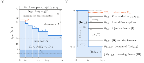
Figure 1 shows the regions that enter: panel (a) the domains of the map flow along the induction, and
panel (b) the step from to .
Figure 1. The regions in the proof of Lemma 5.1, after the rescaling (schematic, not to scale).
(a) Space-time. The map flow is constructed on the shaded staircase: the initial Dirichlet flow lives on
up to the time , and at each time the radius of the domain drops from to . The total decrease of the
radius up to the time is less than , so the domain always contains the ball of the statement (dark).
The equality is used only inside , and the units between the staircase and contain the parabolic balls
of the local Shi estimates. (b) The step from to on the slab . The radius lost in the step is spent in
margins of width , and each property holds on the ball below the corresponding line.
5.2The Step from One Slab to the Next
The next lemma extends the map flow across one time slab and recovers the induction hypothesis on
a domain shrunk by six margins. Its proof is the core of the argument: the extension uses the local
existence statement, a tensor barrier gives a rough metric equivalence and injectivity on the new slab,
and the decay of the Ricci–DeTurck discrepancy on the earlier interval sharpens the equivalence back
to (5.10).
Lemma 5.2 (One-Slab Extension).Let , , and satisfy the hypotheses of Lemma 5.1with ,
and let the constants be as in Section 5.1. There is with the following property. Let and , let
with , and put . If satisfies for the data , then extends to a Ricci–harmonic map heat flow
on that satisfies for the data .
Proof.Extension to the Next Slab. Since , one has
The shrinking-balls lemma [ST21, Lemma 2.2],
under the upper Ricci bound implied by (5.2), gives a dimensional constant such that, for
and ,
whenever the ball on the right lies in . Put and require . Then, for and , the
ball lies in , where the Type-I bound holds. Local Shi estimates for on these parabolic
neighbourhoods, together with complete Shi estimates for , give for , on for the source
and globally for the target,
Choose a smooth domain with
Apply Proposition 2.3(i)
to the time-shifted flows and , at the scale , with initial map and source domain . Its
curvature and first-curvature-derivative hypotheses hold on by (5.13), while (5.10) bounds ;
the source metric and are smooth on a neighbourhood of , since ; and (5.13) gives the
global bounds for the curvature derivatives of on the new slab. Increase , if necessary, so
that . Then (5.12) gives
Hence the corresponding interior set contains . Since by (5.8)
and , the proposition extends to , with on the new slab; the extended map is smooth,
because the two pieces agree at and the equation determines all their time derivatives
there.
Lower Bound and Injectivity. It remains to bound from below and to prove injectivity on a
smaller domain. Write . For one has . Hence Proposition 2.3(ii), applied on that ball, and (5.9) give
on
In particular, since ,
These estimates supply a pointwise tensor barrier. There is such that, if and on at time
then, for satisfying ,
on . The time restriction keeps the lower scalar coefficient positive;
the upper coefficient is automatically positive. To prove the lower bound, fix . At a first
null vector , normalized by , of , differentiating the tensor at fixed gives
At contact
; (5.2), (5.14)–(5.15), and bound every term except in absolute value by . Choosing
makes (5.17) positive, contrary to first contact. Applying the same calculation to , where ,
proves the upper bound. Replacing temporarily by and letting handles non-strict initial
inequalities.
on , so is a local diffeomorphism there. It is
injective on the smaller set . Indeed, suppose for and . Local invertibility defines backward
trajectories by
Here is the spatial differential, and is the time derivative at a fixed source point.
The chain rule gives , so along each trajectory. As long as a trajectory remains in , (5.15) and (5.18)
give
The Type-I bound compares and uniformly on this slab. After integration, the local
distance-distortion estimate between and gives
Choose . The margin of width between and
the boundary of then prevents either trajectory from exiting before . At the induction
hypothesis gives , and uniqueness for the ODE (5.19) gives . Thus is a diffeomorphism onto its
image.
Sharpening and Displacement. It remains to sharpen the rough estimate (5.18) and recover
(5.10)–(5.11). Fix . By the induction hypothesis (5.11), for every ,
Hence is defined on this fixed
target ball. It lies in , where . For a fixed put . The displacement estimate of gives . Since and ,
on this ball. Every point of is of the form with ,
for each , and . So Proposition 2.3(iii), applied at every such with the radius and , gives on , by
(5.9). Thus the hypotheses of Proposition 2.3(iv) hold on the closed cylinder over this ball, centred
at with radius , and applying it with the exponent and evaluating at gives, for ,
Choose a
dimensional so small that
Choose so that the first estimate in (5.20) is at most at . Pulling back at
gives the estimate at for . Since was arbitrary, (5.16), now with and , gives exactly
(5.10) on the new slab over . This is the required estimate on the still smaller domain of
.
Moreover, the gauge identity relating the two flows [Lee26], in which the DeTurck vector field
satisfies , turns the second estimate in (5.20) into
while Proposition 2.3(ii) gives on
the new slab. Measuring the trajectory in , splitting its integral at , and using (5.7), we
obtain, for ,
The first integral converges by the choice of ; on the second one the factor is
absorbed into . By (5.1), (5.21) and the shrinking-balls lemma for ,
Increasing once more
makes the right-hand side of (5.22) at most ; this proves the first line of (5.11) on the new
slab.
Covering. Fix
and put . The definitions and show that lies both in and in the region where
the new displacement estimate holds. Thus, for every , is an embedding on a neighbourhood of and
whereas . Invariance of domain makes open, and compactness of gives . The connected ball does
not meet this boundary and contains ; hence it is contained in . This proves the second
line of (5.11) for the data . Since , properties (I) and (II) hold on as well, so satisfies
.∎
It remains to start the induction, to run it, and to pass from the gauge estimates to the curvature
comparison.
Proof of Lemma 5.1.The Initial Solution. Let be a smooth domain with . On the metrics
and coincide, and so do all their time derivatives and , since both are Ricci flows of the
same metric there and the time derivatives at are determined locally by the initial metric.
Hence the identity map solves the Ricci–harmonic map heat flow to every order at , and the
Dirichlet problem on with initial and boundary value the identity has smooth compatible
data. Short-time existence for this problem is classical [Ham75]; the argument there uses only
the uniform parabolicity of the system and the compactness of and of a target neighbourhood
of it, so it applies to time-dependent metrics. Let be the solution on ; it is smooth up to with
, and its time derivative is bounded on this compact cylinder, so and is uniformly close to
the identity for small . Decreasing therefore makes satisfy for the data : (I) and (II) hold
because a map -close to the identity on the compact set is a diffeomorphism onto its image
with the stated metric equivalence, and (III) follows from and the covering argument at the
end of the proof of Lemma 5.2. The time may depend on the initial geometry; the final time
will not.
The Induction. Put , and . Since the times are geometric,
Choose so small that, whenever , the
total decrease of the radius is less than and ; then and . Decrease below . Repeated application of
Lemma 5.2 gives for every with and : at each step the lemma applies, since and . If instead , the
last step with replaced by any gives for the data . Hence, for every , the flow exists on and
satisfies (I)–(III) for the data of the slab containing : if , and, if , either or with . In the second case
the final time of the data is at most ; in every case it is at most , so the choice of applies to
it.
Conclusion. By the choice of , the ball lies in the region where (III) holds. Restricting
to gives by the displacement estimate, and the second line of (5.11) with centres in
gives . For the final time of the data is at most , so the first line of (5.11) gives the
stated bound. For , the estimate (5.20), which was derived from alone, applied to the
data , and (5.7) give, for ,
The shrinking-balls lemma for and (5.1) then give the same
-displacement bound. This proves (5.3)–(5.4) for a time independent of the initial local
curvature.
The Ricci–DeTurck Estimates. Let , with slab data . Since , the second line of (5.11) with centres
in gives , and for . Hence Proposition 2.3(iii), applied at every with and , gives
after
reducing below . On the metric is a Ricci–DeTurck flow relative to with , and pushing
forward (5.10) from gives the -equivalence there. For the closed ball lies in because , so
Proposition 2.3(iv), with and exponent , gives (5.5) on after a further reduction of . By the
shrinking-balls lemma for , an -ball of fixed radius about each point of stays inside for small .
One-dimensional covariant interpolation along geodesic segments in that ball, using and
followed by polarization, gives
The antisymmetric part of is bounded by . Finally,
which
proves (5.6). Restoring yields the displayed scale factors. All constants depend only on .∎
6Completion of the Bootstrap
The comparison flow of Section 4 and the comparison lemma of Section 5 are now combined. At the
centre of the ball where the two initial metrics agree, for the given flow exceeds the bound of the
comparison flow only by terms that tend to zero with , so it is at most on a time interval
proportional to .
Proof of Proposition 3.1. Let , and be the constants of Section 4.1, and let , and be as in (4.5).
By hypotheses (a), (c) and (d), Lemma 4.1 applies to with . Hence (4.3) and (4.4) hold
for , with and
The Ricci lower bound (3.2) and the local cutoff construction [CC96,
Theorem 6.33], in the form used in [HW22, proof of Lemma 2.2], give a smooth function
with values in , supported in and equal to one on , that satisfies (4.6) with a constant .
Lemma 4.2 therefore gives a domain and a complete metric on it, with constants and
that depend only on and , and Lemma 4.3 gives the Ricci flow of on , where and
.
Put
Then
Since on , the conformal factor is at least one and as quadratic forms on all of ; and
on , so on . This is (5.1). Moreover .
Fix and put . Apply Lemma 5.1 to , , and on , with and ; hypothesis (5.2)
is (6.1). Put . When , (5.3) places in . Diffeomorphism invariance of curvature, (4.12), and
(5.5)–(5.6) give
Here is the norm-comparison factor between and , with , and is the constant of
Lemma 5.1 for .
Choose so that the right-hand side of (6.2) is at most whenever , and also
where is the
constant of Lemma 5.1 for . This choice depends only on . Setting
and using the restriction in
(6.3), the comparison estimate holds for every . Letting proves (3.4). For , the assumed bound gives
We now remove compactness of the initial manifold and prove Theorem 1.3. Throughout this section
is complete and noncompact, , and every point of is a -LRRP, where is fixed in (7.1). We choose
conformal completions whose initial metrics agree with on an exhaustion of . Uniform estimates for
their Ricci flows on one common time interval give a locally smooth diagonal limit, and the
agreement of the initial metrics with on the exhaustion identifies the initial value of that limit with
.
7.1Constants
The conformal change costs a factor close to one in the isoperimetric constant, so the collar estimate
needs slightly more room than was used in Section 4, and the constants are fixed accordingly. Let , ,
and be as in Section 4.1, and let be the conformal profile of Lemma 4.2. Put , and let
be the
constants of Lemma 4.1 for . The constant of Theorem 1.3 is
All these constants depend only on
and .
7.2The Conformal Exhaustion
The first lemma constructs the exhaustion and, for every and every point of , a comparison flow on
the local cover. The conformal change pushes the artificial boundary to infinity, while isoperimetric
control on the local cover survives at the scale of the original metric, which becomes a fixed scale for
the conformal metric. This scale tends to zero towards , so the construction uses the LRRP condition
at all scales below .
Lemma 7.1 (Uniform Conformal Exhaustion).There are relatively compact domains with smooth
boundary, compact sets whose union is , and smooth functions on such that is a complete metric
of bounded curvature on and
Moreover, there are , depending only on , with the following property.
For every and every , let on the part of the local cover that lies over . There are an
open set in this part and a complete bounded-curvature Ricci flow on such that, with ,
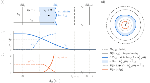
Figure 2. The conformal exhaustion of Lemma 7.1 (schematic, not to scale). Panels (a)–(c) show the
construction along a ray from the base point . (a) The regions. The metric equals where , in particular
on ; the boundary of is at infinite distance for it, and lies in the interior of the next compact set .
(b) The cutoff , the regular value that defines as a superlevel set, and the defining function . (c) The
conformal exponent , which vanishes where and tends to infinity at , and the function , which is
Lipschitz and vanishes there. (d) The local cover at a point , with the metric ; balls without a subscript
are taken for this metric. The second completion takes place at the fixed scale , inside the ball of the
lifted original metric, where ; the radius of this ball tends to zero as approaches . It produces the
domain and the complete metric that starts the comparison flow.
Proof.The Exhaustion. Fix and , and put . We first construct a cutoff at unit scale, as in
[HW22, proof of Lemma 2.2]. Let be a maximal subset of whose points are pairwise
at distance at least ; it is finite because is compact. The balls cover , and the balls
are disjoint. By the Bishop–Gromov inequality, every point of lies in at most of the
balls . The Ricci lower bound gives smooth cutoffs with
[CC96, Theorem 6.33]. Fix
a smooth nondecreasing with and on , and put . Then
Choose a regular value of ,
let be the component of containing , and put on , with the function of the proof of
Lemma 4.2,
Thus vanishes on , tends to one at , and satisfies
As in the proof of Lemma 4.2,
the last inequality in (4.10) and (7.4) show that every curve leaving compact subsets of
has infinite -length, so is complete, and has bounded curvature because and extend
smoothly past the compact set . Since
this gives (7.2). Figure 2 shows these regions and
functions.
Uniform Bounds. By (4.9), (7.4), the conformal scalar-curvature formula, and the bound , there is
a constant such that
Indeed the derivatives of occur only in the combinations of (4.9), and only the
Laplacian of , not its full Hessian, enters the scalar-curvature formula.
So is -Lipschitz for
along curves in , and it extends continuously by zero to . Hence , and for every with ,
Isoperimetry on the Cover. Require
Since , the closed ball of radius about in the local cover is
compact, by Lemma 2.1; the Ricci lower bound gives ; and the LRRP condition at gives
So
Lemma 4.1 applies to at , with and : every regular domain satisfies
The Conformal Metric on the Cover. Put and require . By (7.6) with , the ball lies over , its
closure is compact, and on it the lift of , still written , satisfies . Comparing boundary areas and
volumes for and , we get from (7.7), for every regular domain ,
Since , we may decrease so that the
constant on the right is at least . Set
and decrease once more so that . A curve from to the
boundary of has length at least for , hence at least for . Therefore , the closed -ball of radius about
is compact, and by (7.5)
while by (7.8) every regular domain satisfies (4.4) for the metric , with
.
The Cutoff on the Cover. The local cutoff construction [CC96, Theorem 6.33] for the metric ,
whose Ricci curvature is at least , gives a smooth function with values in such that
where the
derivatives are taken for and . The conformal Laplacian identity
with . By the two-sided bound for on , the -distance from to the
complement of is at least , and every point of is at -distance at most from , because . Hence
The Comparison Flow. By (7.9), the isoperimetric inequality stated after it, (7.10) and (7.11),
Lemma 4.2 applies to the metric , the point and the radius , with . It gives a domain with
and a
complete metric of bounded curvature on that dominates , agrees with it on , and satisfies the
hypotheses of Lemma 4.3 with , where is the constant of Lemma 4.2 for . Panel (d) of
Figure 2 shows these regions. Let be the flow of this metric given by Lemma 4.3. It
exists on with
and it satisfies the last line of (7.3). Since , the other two lines hold as
well.∎
7.3Uniform Lifetime
The second lemma is the first-time argument of Section 3 for the flows of the exhaustion metrics,
with the flows of Lemma 7.1 as comparison flows.
Lemma 7.2 (Uniform Lifetime of the Exhaustion Flows).There is such that, for every , the
complete bounded-curvature Ricci flow with exists on and satisfies
Proof.Shi’s theorem [Shi89] starts a maximal complete bounded-curvature flow from each ; its
lifetime may depend on . Define
This number is positive for each .
Fix and lift to the part of the local cover that lies over . On every interval with , the lifted flow
and the comparison flow satisfy the hypotheses of Lemma 5.1 with , , and : the first line of (7.3)
gives , (5.1) is its second line, and (5.2) follows from the definition of and its third line. As in the
proof of Proposition 3.1, with and , this gives
for . Choose so that the right-hand side is at most
for and , and put
Then, for every ,
Suppose . If , the strict margin in (7.13) extends the defining
inequality of past ; the required continuity of the curvature supremum follows from the global
derivative estimates of Shi on every compact subinterval of positive time. If , (7.13) bounds the
curvature on the final half of the maximal interval, and the continuation theorem for complete
bounded-curvature flows extends the flow. Both alternatives are impossible. Hence , and (7.12)
follows.∎
7.4The Limit Flow
The third lemma passes to the limit. It follows the compactness argument of Simon and Topping
[ST21, Section 8, proof of Theorem 1.7]. Their existence theorem is three-dimensional and comes
with a Ricci lower bound for positive time, but the two local estimates that it invokes and its
diagonal extraction need neither.
Lemma 7.3 (Exhaustion Limit).After passing to a subsequence, the flows converge locally
smoothly on to a complete Ricci flow with and
Proof.Fix and a radius with , for the compact sets of the proof of Lemma 7.1. Then
For all
sufficiently large , on a neighbourhood of . Since , the -ball of radius about a point is then
contained in , so the curvature of is at most on it. The flow is complete, so its balls are relatively
compact in , and it satisfies (7.12) with . These are the hypotheses of [Che09, Theorem 3.1], in
the form recorded as [ST21, Lemma 8.1], at every centre . Its conclusion at the centre
is
for all large . The initial curvature derivatives are uniformly bounded on , because
the initial metric there is exactly . Since is a compact neighbourhood of , (7.14) and
the local derivative estimate [ST21, Lemma 8.2] give uniform bounds for all curvature
derivatives on . Working in fixed coordinate charts, as in [ST21, Section 8, paragraph following
Lemma 8.2], Arzelà–Ascoli gives a smooth subsequential limit on . A diagonal argument over
produces a smooth Ricci flow on all of . Since the initial metrics are equal to on every fixed
compact set for all large , the convergence includes and . Estimate (7.12) passes to the
limit.
It remains to check completeness. The shrinking-balls lemma [ST21, Lemma 2.2], applied to the
complete flow with (7.12) and with arbitrarily large radii, gives, for a constant and all ,
For any
curve in from to , local smooth convergence and (7.15) give
Taking the infimum over
such curves gives the same lower bound for . Thus every -ball about a fixed base point is
contained in a compact -ball, and the Hopf–Rinow theorem implies that is complete for every
.∎
The comparison lemma also gives the uniqueness part of Theorem 1.3.
Corollary 7.4 (Complete Type-I Uniqueness).Let and be complete Ricci flows, smooth on
, with the same complete smooth initial metric . If on for some , then on .
Proof.Fix a point in a connected component. For all sufficiently large , apply Lemma 5.1 with , ,
and ; each of the two curvature norms is at most . Completeness of gives the compact balls required
there, and , so the conclusions hold for . The resulting maps are defined on , satisfy , and obey
The
first estimate keeps the images of each compact source set in a fixed compact target set,
independently of , while (5.4) uniformly bounds . On a positive-time compact cylinder,
Proposition 2.3(ii) and interior parabolic regularity give uniform derivatives of . Diagonal
extraction therefore gives a smooth Ricci–harmonic map heat flow on , continuous at
with . For any fixed compact set, its images lie in for large . Pulling back the second
estimate, with only a uniform factor from (5.4), and taking the limit gives . Thus is a local
isometry, so its covariant Hessian and tension vanish. The Ricci–harmonic equation gives ;
continuity at forces and hence for , and at by continuity. Apply the argument on each
component.∎
Proof of Theorem 1.3. Set , and recall that by (7.1). If is closed, existence is Theorem 1.2 and
uniqueness is Hamilton’s uniqueness theorem for closed manifolds [Ham82]. If is noncompact,
Lemmas 7.1 to 7.3 give the flow on . If two complete flows with initial metric satisfy a bound
, the sum of their curvature norms is at most , and the two flows coincide by Corollary 7.4.∎
8Singular Nilpotent Fibrations
At one fixed positive time, Theorem 1.2 supplies bounded-curvature metrics. The distance distortion
estimate of [HW22, Appendix A] identifies their limit bi-Hölder homeomorphically with the original
one, and the theory of Fukaya and Cheeger–Fukaya–Gromov supplies the fibration that we transport
across this homeomorphism.
8.1The Fibration Theorem for Bounded Curvature
We use the theorem of Fukaya [Fuk87], [Fuk89, Theorem 9-1] and Cheeger–Fukaya–Gromov [CFG92]
in the form of [Ron26b, Theorem 1.13]. For a metric , equip with its canonical metric, so that acts
isometrically and .
Theorem 8.1 (Nilpotent Fibrations under Bounded Curvature).Let be closed -manifolds with converging in the Gromov–Hausdorff topology to a compact metric space with and . After passing to
a subsequence, for a closed manifold carrying a Riemannian metric with Hölder continuous first
derivatives and an isometric -action. For large there is an -equivariant fibre bundle whose fibre is
a nilmanifold and whose structure group is affine, inducing a continuous map in the
diagram
Every fibre of is a positive-dimensional infranilmanifold. Moreover, for some
,
(i)
both and are -Gromov–Hausdorff approximations;
(ii)
for orthogonal to a fibre;
(iii)
the fibres of have second fundamental form at most .
8.2The Precise Statement
The parameter below governs the Hölder exponents relating the two limits.
Theorem 8.2 (Singular Nilpotent Fibrations, Precise Form).Fix , and , and put
where is the
constant of Theorem 1.2. There is with the following property. Let be closed -manifolds with and
uniform -LRRP, converging in the Gromov–Hausdorff topology to a compact metric space of positive
diameter, with . Let be the Ricci flow with , and put . Then every subsequence has a further
subsequence along which the following hold.
(a)
The sequence satisfies the hypotheses of Theorem 8.1for some limit . Let , , and be as in that theorem.
(b)
There is a homeomorphism , the limit of the identity maps , such that and are Hölder continuous, with exponents and and with constants depending only on , and .
(c)
The maps
are continuous and surjective, every fibre of is an infranilmanifold of positive dimension, and is an -Gromov–Hausdorff approximation from to , with .
Consequently, for every , all but finitely many of the original sequence carry a map of this
kind that is an -Gromov–Hausdorff approximation from to , with satisfying (i)–(iii) of
Theorem 8.1for in place of . Here , , and may depend on , and the constants in (b) do
not.
Thus fits into (8.1), with identified with through . The estimates of Theorem 8.1 use
the canonical metric of ; the - and -frame bundles are -equivariantly diffeomorphic via
.
8.3Uniform Bi-Hölder Distortion
The Ricci flow enters only through this comparison at one fixed time.
Lemma 8.3 (Uniform Bi-Hölder Distortion).Let be as in Theorem 8.2. There are and ,
depending only on , with the following property. Let be closed with and uniform -LRRP, let be its
Ricci flow, and put , , and . Then , , and for all
Proof.Put , where is given by Theorem 1.2. Its curvature estimate implies
The scalar lower bound
persists by the maximum principle, since is closed, and Bishop–Gromov and Buser’s inequality
[Bus82] give dimensional doubling and Poincaré constants on balls of radius at most . Thus
[HW22, Theorem A.1], applied with arbitrary base point and coefficient , gives and such
that, for and ,
Here ; we use the estimate obtained at the end of the proof of [HW22,
Theorem A.1].
Set , so that and . After taking and enlarging , the upper half of (8.5) gives (8.2). Subdividing a
minimal -geodesic into arcs of length at most gives and hence (8.4), after enlarging
.
Put . If but , continuity of along a minimizing -geodesic gives a point with , and (8.5) gives the
contradiction . Thus the lower half of (8.5) applies to and yields (8.3) after shrinking and enlarging
.
We now identify the two limits and transport the fibrations of the smoothed metrics.
Proof of Theorem 8.2. Let be the constants of Lemma 8.3. Write and , and fix
-Gromov–Hausdorff approximations with . We start from a given subsequence and pass to
further subsequences without changing the notation.
The Smoothed Limit. By Lemma 8.3, , and (8.4) bounds the diameter of by for large. By
Gromov’s precompactness theorem, a subsequence of converges to a compact metric space . Since ,
the sequence collapses and [CC97, Theorem 3.1]. Choose with . By (8.3),
so . Thus Theorem 8.1
applies and gives (a). In particular the maps are continuous, surjective -Gromov–Hausdorff
approximations from to , after enlarging .
The Homeomorphism. For choose with , so that
On a countable dense set , compactness and a
diagonal subsequence define
The first holds when , and the second when the corresponding -distance is less than .
Thus extends continuously to , both inequalities persist under these restrictions, and is
injective.
We claim that
Indeed, fix and a finite -dense set . For large , and the defining convergence is
within on . Given , choose with . Then , and (8.2), (8.7), and the triangle inequality bound the
distance in (8.9) by . Letting proves the claim.
Since is surjective, (8.9) makes the compact set dense in . Thus is a homeomorphism, with the
global Hölder bounds in (b) following from (8.7)–(8.8) and the diameter bounds.
The Fibrations. Put . It is continuous and surjective with the same positive-dimensional
infranilmanifold fibres, and (8.9) and (8.8) give
Hence is an -Gromov–Hausdorff approximation, where is plus twice this supremum, and its diagram is (8.1) composed with .
Finally, if the whole-sequence assertion failed for some , its bad subsequence would have a good
further subsequence by the argument above, a contradiction.∎
Proof of Theorem 1.4. Apply Theorem 8.2 with , so that . By its last assertion there are
indices such that every with carries a map of the kind described there that is a
-Gromov–Hausdorff approximation. For choose such a map and put . Properties (i) and (ii)
are part (c) of Theorem 8.2, and (iii) is the diagram (8.1), in which the manifold may depend
on .∎
8.5A Consequence for Aspherical Manifolds
The homeomorphism transfers the topological conclusion of [Ron26b, Conjecture 0.7] under the
hypotheses of case (0.6.1) of [Ron26b, Conjecture 0.6].
Corollary 8.4 (Aspherical Limits).Let and be as in Theorem 1.4. If every is aspherical
and its fundamental group is of type in the sense of [Ron26b, Definition 0.4], then is
homeomorphic to an aspherical manifold.
Proof.Apply Theorem 8.2 with . The bounded-curvature sequence collapses to with positive
diameter, so [Ron26b, Theorem A] makes an aspherical manifold; now use .∎
9A Counterexample under Rewinding Volume Control
This section proves Theorem 1.5 and Corollary 1.6 independently of Sections 3 to 8, using the
properties of Nifa’s manifolds listed below.
9.1Nifa’s Sequence
After the subsequences in [Nif26, Theorem 1.3], write for Nifa’s pointed sequence and its limit. In
[Nif26] they are denoted and . Write for the cone over and for the circle of length ; the parameter
is denoted in [Nif26]. We use exactly the following cited properties.
(N1)
The Sequence. Each is a closed four-manifold, and there are with
The space is compact, and the convergence is realized by isometric embeddings of all and of into one compact metric space, called the ambient space below, in which in the Hausdorff distance and [Nif26, Theorem 1.3, Lemma 9.3, proof of Proposition 2.3].
(N2)
The Singular Point. The tangent cone of at is unique and equal to , where . The inclusion of any neighbourhood of into induces a map on whose image has infinite rank; in particular is not locally contractible at [Nif26, Theorem 1.3 and (7.1)].
(N3)
The Cores. There are compact Riemannian four-manifolds with boundary , , each diffeomorphic to minus an open ball, such that for all the manifold contains an isometric copy of as a smooth domain, and the copies of different in are disjoint [Nif26, (9.3)]. Let , a closed topological four-manifold homeomorphic to , with base point the image of , and let be the quotient map on and the constant map to on .
(N4)
The Limit Maps. There are continuous maps and such that is the quotient map, is injective on , the inclusions converge to uniformly in the ambient space as , and whenever in the ambient space [Nif26, Proposition 2.3 and its proof, Lemma 2.5].
(N5)
The Regular Part. The set is a connected topological four-manifold. It carries a smooth structure and a smooth Riemannian metric such that every point of has a neighbourhood on which is the distance of . Moreover there are a compact domain with nonempty interior and smooth embeddings such that in and converges to the inclusion of uniformly in the ambient space [Nif26, Lemma 14.1 and its proof].
Two consequences of (N3)–(N4) will be used. For and ,
Indeed, for , one of the two disjoint cores
is avoided along a subsequence, and the corresponding quotient converges to . Also
The reverse inclusion follows because is the quotient map. For the forward inclusion, an approximating sequence
for a point with eventually lies in a compact subset of ; the inverse is composed with the inverse of
the quotient there. Thus is a homeomorphism, and is an open four-manifold, disjoint from by
(N2).
The lower bound for the Reifenberg constant also uses the shape of near the base point. The next
lemma extracts what is needed from the construction.
Lemma 9.1 (Simply Connected Neighbourhoods of the Base Point).There are numbers and a
constant such that for all there is an open, connected and simply connected set with
Proof.We use the construction of [Nif26, Section 14], in which for all and is obtained from
the unit sphere by replacing disjoint round balls with the cores of (N3). Let be the round
distance, and let be the numbers of the proof of [Nif26, Lemma 14.1]. They satisfy , the round
ball that replaces is centred at -distance from , and the open -ball of radius about contains
the round balls replaced by for and is disjoint from those replaced by for [Nif26, Section 14
and the proof of Lemma 14.1]. Let be the open set obtained from this ball by the replacements
of index made in . It is connected and simply connected by van Kampen, since finitely many
disjoint balls are replaced by copies of minus a ball.
Let be the function on given by [Nif26, Lemma 13.2], where it is denoted . It vanishes
at , it is -Lipschitz, it equals on , it lies between one half and twice outside the , and for
a constant independent of [Nif26, Lemma 13.2, (13.5) and (13.6)]. Moreover on [Nif26,
(14.4)]. Outside , a point lies either on some with , where , or outside the at -distance at least
from ; in both cases . Since , every point at distance less than from lies in , and every point
of is at distance at most from . This proves the inclusions with .∎
9.2The Products
Let , with , and equip
with the product metric; write for the image of . The next proposition verifies
for the hypotheses of the statements recalled in the introduction.
Proposition 9.2 (The Hypotheses).Put and .
(a)
.
(b)
Every point of every is a -LRVP.
(c)
and . Hence and .
Proof.(a) The circle factor is flat and .
(b) By Myers’ theorem and (N1), . For the ball contains , and the Bishop–Gromov inequality for
gives
For , let be the component over in containing . Since , the connected cylinder lies in , and
its rectangle with lies in the intrinsic unit ball about . The local-isometric cover maps the unit
ball about onto that ball by path lifting. Writing for the product metric, (9.3) gives
(c) The projection is onto and changes distances by at most the diameter of the circle. By the
Bishop inequality, .∎
9.3No Continuous Approximation
The obstruction is topological and concerns only .
Theorem 9.3 (No Continuous Approximation, General Form).There are and such
that for
The same holds, with the same and , for every continuous map and every
.
All degrees below are modulo two. For a proper map between four-manifolds, write for the image
of the fundamental class around the compact preimage of in the target’s local homology . It is
locally constant in , and on closed connected four-manifolds it is the multiplier on [Dol95,
Chapter VIII, §4]. The degree over a point is detected by the following form of the Borsuk–Ulam
theorem.
Lemma 9.4 (Borsuk).Let a continuous map from the closed ball to take distinct values at
any two points whose distance is at least . Then the image of the centre is not in the image of
the boundary sphere, and the degree of the map over the image of the centre is odd.
Proof.Denote the map by . For and we have , so . Thus the normalized map below is always
defined; at it also shows that is missed by the boundary and gives the degree map over :
At
this map is odd, so its degree, and hence the degree of over , is odd.∎
With it, a continuous map of small distortion is shown to have degree one over the regular part of
.
Lemma 9.5 (The Degree Is One).There are and such that for and every continuous with , the
proper map
has .
Proof.The restricted map is proper because the preimage of a compact subset of is closed in
. Its target is a connected four-manifold by (N5), so it suffices to find one point over which the
degree is one.
Fix two points in the interior of and smooth coordinate charts of centred at them, with
domains in the interior of . By (N5), as in the proof of [Nif26, Lemma 14.1], there are ,
and such that for the composition of the inverse of the chart at with is defined on
and satisfies
and the same holds for the chart at . Put . By (N5) there is with for
.
The set of points of at distance at least from is a compact subset of the manifold . By the
Lebesgue number lemma there is such that every ball about a point of this set lies in an open
subset of homeomorphic to . Choose
Let and . The images of and under are at distance more than , so they are not both within of .
Say is at distance at least from , and let be an open set homeomorphic to that contains . Consider
on the closed ball of radius . Its image lies in . If , then , so . By Lemma 9.4, applied in , the degree
of over is odd. Finally, every point of is within of in . Since , it lies in , and its coordinate has
norm less than . So , and .∎
Proof of Theorem 9.3. Let be as in Lemma 9.5, let , and suppose that is continuous with . For
put
where generates . Here runs over all positive integers, not only over the cores present in : the
maps are defined on .
Squares. Let , and let be its preimage under . By (9.2), , and is a homeomorphism near . So by
Lemma 9.5. Since generates ,
Products. For the map takes values in the wedge , by (9.1). The class restricts to zero on the
wedge, because it vanishes on each of the two factors. Hence on , and .
Count. If is a finite relation with , multiplication by gives , so . The classes are therefore
linearly independent in , which is finite-dimensional. This is a contradiction.
For the product, restrict a continuous map to a slice . The slice carries the distance of , so the
restriction has distortion at most .∎
9.4The Limit Is Not an Orbit Space
The limit cannot be the compact-group quotient occurring in a Cheeger–Fukaya–Gromov
fibration.
Proposition 9.6 (Orbit Spaces Are Locally Contractible).Let a compact Lie group act
smoothly on a smooth manifold . Then is locally contractible. Consequently is not
homeomorphic to for any such and .
Proof.By the slice theorem [Bre72, Chapter VI, Section 2], a neighbourhood of is modelled
on a neighbourhood of in . A -invariant ball in contracts equivariantly to , so its quotient
contracts; such quotients form a neighbourhood basis. Apply (N2).∎
9.5The Reifenberg Constant: Upper Bound
We quantify the facts that a ball in the local cover of a product contains a line segment through its
centre and obeys Bishop–Gromov comparison.
Lemma 9.7 (A Crude Correspondence).Let be a metric space with a point such that for all . Let
, let be integers, and suppose that
(a)
is the union of sets of diameter at most ;
(b)
there are with and for ;
(c)
is the union of sets of diameter at most ;
(d)
there are with and for .
Then there is a correspondence between and that contains and has distortion at most . Hence the
pointed Gromov–Hausdorff distance between and is at most .
Proof.Let be the sets in (a) and those in (c), made disjoint. Relate to if , relate to if ,
and relate to . Both projections are onto. For two pairs from the first rule, equal indices give
distortion at most by radial convexity and (a), while unequal indices compare numbers in
and . The second rule is symmetric. For one pair of each kind, both distances are less than ;
a pair with compares numbers in . Thus the distortion is at most , and the pointed bound
follows from Section 2.1.∎
The next lemma bounds the number of sets needed in hypothesis (c).
Lemma 9.8 (Covering by Radial Retraction).Let be a complete Riemannian manifold with , let and , and let with . Then the ball in the local cover is the union of at most
sets of diameter less
than .
Proof.Put and write for the lifted distance. Radially retract along a minimizing geodesic, available
by Lemma 2.1, to at distance from . Then
Let be a maximal -separated subset of . The balls of
radius about the cover , and their radial preimages have diameter less than . The -balls are disjoint.
If has the least such volume, their union lies in ; moreover has depth at least . Hence
Lemma 2.1 (iii) gives
∎
The two lemmas give the upper bound.
Proposition 9.9 (The Upper Bound).Let be a complete Riemannian manifold with , let ,
and let with the product metric. For every , every and every , the pointed Gromov–Hausdorff
distance between the ball of radius about in the local cover at and is at most . In particular
every point of is a -LRRP for every and every .
Proof.We verify the hypotheses of Lemma 9.7 with , , , and the ball of radius about in
the local cover at . For (a), the ten sets cover and have diameter at most : in the first set, .
For (b), the circle projection lifts to a -Lipschitz function on with along the arclength lift
from , for . Thus the lifted-circle points , , are pairwise -separated and lie within of . For
(c), Lemma 9.8 with gives sets. Finally, the points with and verify (d), since they are
-separated and lie in the ball of radius . Thus Lemma 9.7 gives .∎
9.6The Reifenberg Constant: Lower Bound
A quantitative Borsuk–Ulam theorem separates the tangent model from .
Lemma 9.10 (Local Covers of Products).Let be a closed Riemannian manifold, , and . Let
, and suppose that is contained in a connected and simply connected set of diameter less than
. Then the ball of radius about in the cover is isometric to the ball of radius about in with
the product distance, by an isometry that takes to .
Proof.Let be the component over in containing . The local cover factors through a local
isometry , and contains the product -ball. Product geodesics between points of the -ball have
length below and remain in the -ball, so the product and intrinsic distances agree there; the
same argument from identifies the intrinsic and product balls of radius at most . Moreover
every loop in the -ball lies in the simply connected set and hence lifts closed. Path lifting
therefore maps the -ball about onto the product -ball. Given two lifted points, join their
images by paths of length tending to their product distance; the resulting loops with paths
from the base point lie in the -ball and lift closed, so the lifted distance is no larger. The reverse
inequality follows from local isometry.∎
We use unpointed Gromov–Hausdorff distance below; it is no larger than the pointed distance in
(1.1).
Proposition 9.11 (The Model).Let , and let be the closed unit ball of about a point of the
singular axis, with the restricted distance. Put , and let be the smallest positive root of
Then the
Gromov–Hausdorff distance between and the closed unit ball of is at least . The function is
decreasing, with
Proof.Let be a correspondence between the closed unit ball of and with distortion at most ; we
may assume . For choose a point of that is related to , and write it as , with and in the cone at
distance from the vertex. Points of satisfy , and the distance of two of them is given by
where is
the angle between the directions of and . Put . Then, for and the distance of the two chosen points,
Antipodes. For and the distance of the chosen points is at least . Since the cosine above is
nonnegative and , we get , that is, . By (9.4),
Jumps. If , the inequality obtained below is trivial, so assume . The map
from to sends
antipodes to antipodes. By the theorem of Dubins and Schwarz [DS81], in the form of [LMS23,
Corollary 5.3], its modulus of discontinuity is at least : for every there are , arbitrarily close to each other, whose images are at distance at least . On the other hand, by (9.4) and the distortion
bound,
and the same holds at the antipodes. So the numerator changes by at most
between and . Its norm is at least , and the radial projection onto the sphere of radius
does not increase distances outside that sphere, so the images of and are at distance
at most . Hence , that is, . Written out, the quadratic polynomial in the statement is
nonnegative at , and it is negative at . So , and the Gromov–Hausdorff distance is half
the infimum of the distortions. For fixed the polynomial increases with , so its smallest
positive root decreases as increases. The numerical values follow from the formula for the
root.∎
Together with the construction, Proposition 9.11 gives the lower bound in part (v) of
Theorem 1.5.
Proposition 9.12 (The Lower Bound).For every and every there is such that for the
point is not a -LRRP. In particular, for no and no do all the have uniform -LRRP.
Proof.By Lemma 9.1 choose with , and let . For the ball lies in the connected and simply
connected set , whose diameter is less than . By Lemma 9.10 the ball of radius about in the local
cover at is isometric to the ball of radius about in . By (N1), as these balls converge in the
Gromov–Hausdorff distance to the ball of radius about in . By (N2), as the latter balls, rescaled by
, converge to . Therefore, by Proposition 9.11,
where is the metric of and the distance
may be taken unpointed. This proves the first assertion. The second follows because by
(N2).∎
Proof of Theorem 1.5. Parts (i) and (ii) are Proposition 9.2; the diameter of is positive
because has a tangent cone of dimension four. Part (iii) is Theorem 9.3. Part (iv) is (N2)
and Proposition 9.6. Part (v) is Proposition 9.9, applied to , and Proposition 9.12.∎
Proof of Corollary 1.6. By parts (i) and (ii) of Theorem 1.5, the are closed five-manifolds
with and uniform -LRVP that collapse with vanishing volume to the compact,
positive-diameter limit , which has dimension four. Thus they satisfy the common hypotheses
of the LRVP statements recalled in the introduction. A singular nilpotent fibration in the sense
of [Ron26b, Section 1.3] is, in particular, a continuous -Gromov–Hausdorff approximation with
: the frame-bundle map in (8.1) is one, and the vertical maps are quotients by isometric actions.
So each of the statements (a)–(d) would provide, for all large , a continuous -Gromov–Hausdorff
approximation with . This contradicts part (iii) of Theorem 1.5. The last clause of (a) follows
from part (v).∎
Remark 9.13 (Other Dimensions). Replacing the circle by , with , and using the radius in
place of in the proof of Proposition 9.2 gives uniform -LRVP for some , and hence analogues
of parts (i)–(iv) of Theorem 1.5 and of Corollary 1.6 in every dimension ; the obstruction
follows by restriction to a slice.
10Discussion
10.1Between the Two Thresholds
In dimension five, Theorems 1.4 and 1.5 leave open the range between and . The upper estimate of
Proposition 9.9 is automatic for the circle products, whereas Proposition 9.11 shows that the conical
model cannot produce a counterexample below when its cone angle is at most . A smaller
counterexample would need a larger angle or a different mechanism. It is also open whether a
positive threshold can be chosen independently of dimension, or whether can arise from
another Ricci-lower-bounded sequence with uniform LRVP that does admit continuous
approximations.
10.2Neighbouring Cases
The example of [Ron26b, Example 4.2] has no singular nilpotent fibration but does admit
continuous approximations, so it does not decide parts (b)–(c) of Corollary 1.6: use the
residual-circle orbit map and collapse the two small two-spheres over the poles to the vertices. The
sectional-curvature case (0.6.2) of [Ron26b, Conjecture 0.6], with , also remains open:
such limits are locally contractible Alexandrov spaces [Kap06], unlike , while sectional
lower bounds and LRVP do not imply small-constant LRRP, as shown by products of
a shrinking circle with smooth convex surfaces converging to a surface with a conical
point.
Acknowledgments and Tool Disclosure. The author used Anthropic’s Claude and OpenAI’s Codex for drafting and restructuring the
exposition, for checking the arguments against the cited sources, for the numerical evaluation of the
constants in Section 9, and for the preparation of the figures. The author takes full responsibility for
the mathematical claims and the exposition.
ALocal Ricci–Harmonic Comparison Estimates
This appendix proves parts (i)–(iii) of Proposition 2.3. Lemma A.1 constructs the map heat
flow on a conformal completion of the source; its existence time depends only on and ,
and the bounds of the construction that depend on the geometry enter only through the
short-time existence lemma of [BK22]. Lemmas A.2 and A.3 give the interior derivative
bounds.
A.1Interior Existence and Uniform Continuation
The flow is first constructed on a conformal completion of the source domain, and a comparison for
its energy density makes the existence time uniform.
Lemma A.1 (Interior Existence).Under the hypotheses of Proposition 2.3(i), its conclusion
holds with in place of .
Proof.Rescale . We use a fixed conformal completion of the source, as in [Hoc16; Lee26],
and verify the bounds needed for a moving source. On a component with empty boundary
take ; compactness gives all the qualitative bounds below. The following construction is for
components with boundary.
Put , with paths in . For and , let be a normalized smooth radial kernel on in
and set
the Riemannian convolution of Greene and Wu [GW79]. These geodesics remain
in , and the curvature bound excludes conjugate points along them; since the integral
is taken over the tangent space, no bound on the injectivity radius enters. We use the
estimates
The first is the Lipschitz bound on . For the others, work in an orthonormal
trivialization that is parallel at , and write
Differentiating a smooth Lipschitz approximation of
twice in the centre produces
where is the covariant second centre variation. Since , the
Hessian term is a vertical derivative along minus , and integration by parts in gives
The Jacobi equation and its first variation, together with the normalization
bound , ,
and , and . Since , this proves (A.1), also in the limit for the distance function itself.
Writing with a kernel that is smooth in , because vanishes to all orders at , shows that is
smooth; repeated centre differentiation and vertical integration by parts, with , give , where
for also depends on the curvature derivatives of the compact smooth extension of the
metric.
Take and a fixed smooth nondecreasing function equal to zero below and one above . Define
Each summand is defined where and extended by zero; it already vanishes for , so is smooth. Only
a bounded number of scales have nonzero derivatives at a point, and the smaller-scale
tail is locally constant. Consequently
Also on . The constants for may depend on the
geometry.
The source assumptions give . For a dimensional , integration of the metric and connection
equations gives and for . Thus (A.2) holds with -derivatives as well. Fix a smooth nonnegative
nonincreasing function with for and for , and set
Then , on , and is complete because near . The conformal curvature formula gives
Indeed and .
All the following bounds are finite:
For the first term, use derivatives of through order ; the
second also uses derivatives of through order . All are available from the compact smooth extension
and (A.2). Their boundary weights are respectively and , which are bounded. Unlike (A.3), these
bounds depend on the geometry of the extension; they enter only through [BK22] below. The target
Ricci flow has bounds of the same kind by hypothesis.
Now is -Lipschitz, and [BK22, Lemma A.8] gives a solution for the two complete evolving metric
families on a short time interval, whose length may depend on (A.4). For , take a -orthonormal frame
. The Bochner identity for moving metrics is
where when span a positively curved plane. By (A.3)
and , . The maximum principle for bounded solutions on these complete families with bounded
geometry, as in [BK22, proof of Lemma A.6], compares with the solution of , . Thus up to
Let . The bounds (A.4) and those of the target are uniform on , and for , so at every time
[BK22, Lemma A.8] supplies the same positive existence time for the initial map . Restart
within the preceding existence interval and concatenate: the two solutions agree at the
joining time, and the equation determines all their time derivatives there from the spatial
derivatives of the common map, so the one-sided jets match and the concatenation is smooth.
The energy comparison on every finite concatenation continues to use the original initial
time and gives . Finitely many restarts cover . Restrict to , where , and restore the scale
.∎
A.2Covariant Map Derivatives
The interior derivative bounds follow from a Shi-type induction on the covariant derivatives of the
map.
Lemma A.2 (Local Map Derivatives).Let be a Ricci flow on an open -manifold and a
complete Ricci flow on an -manifold . Suppose and
If is a smooth Ricci–harmonic map heat
flow on this source cylinder with , then, for every integer ,
on for , where depend only on .
Proof.Rescale and enlarge to . Local Shi estimates give, for a common smaller time and through
order ,
by the shrinking-balls lemma [ST21, Lemma 2.2], the parabolic neighbourhoods of radius
used on stay inside . Complete Shi estimates give the same bounds for all target curvature
derivatives.
Put , and let denote target covariant differentiation along in time, leaving the source indices
unchanged. For a tensor with covariant source slots and one target slot,
the sum running over the
source slots. The Ricci endomorphisms act on the indicated source slot and on the target slot,
respectively; the target tensor is pulled back along . Spatial metric compatibility therefore gives
Commuting through the tension field, and using that is a universal contraction of and ,
together with the target analogue, gives universal contractions of the forms
The number of factors
depends only on , and the factors are bounded. These relations follow inductively: a derivative either
raises a curvature order or a jet index, with an extra undifferentiated when it differentiates target
curvature. The moving-target connection terms have the same relations. Consequently, if
for ,
Terms containing have curvature order zero and only as other jet factors; all
other terms are controlled by the lower jets. For the same bound follows directly using
.
Suppose the bounds hold through . Equations (A.6)–(A.7) and Young’s inequality imply
For the localization take . At the step from to , centre a cutoff at and put . A nonincreasing
distance cutoff
has compact support in , equals one at for a common smaller time, and satisfies
Here is a fixed smooth nonincreasing function equal to one below and zero above , with and . The
shifted distance is a parabolic supersolution on the transition annulus, and by the shrinking-balls
lemma the support stays in . At cut points the calculation is understood in the barrier
sense.
Consider . At a positive-time interior maximum, (A.8)–(A.9) give
The last term is at
most . For and large , it follows that at the maximum. On the lateral boundary and is
already bounded. At the second term vanishes; the first is bounded by when and vanishes
otherwise, since is smooth on the closed cylinder. Thus the maximum principle bounds ,
and gives . The constants are uniform in . Induction reaches . Restoring proves the
statement.∎
A.3Ricci–DeTurck Derivatives
The derivative bounds for the Ricci–DeTurck flow are the map derivative bounds of Lemma A.2 in
disguise: the gauge identity below expresses the covariant derivatives of through the Hessian of
.
Lemma A.3 (DeTurck Derivatives from Map Derivatives).Let , , , , and be as in
Lemma A.2, and suppose that every is a diffeomorphism onto its image with on for some .
Then satisfies, for every integer ,
on for , where depends only on and is the constant of
Lemma A.2.
Proof.Fix and write , a metric on for which is an isometry onto its image, and . Pull-back
commutes with covariant differentiation, so
The two connections on the source are related
through the Hessian of : since intertwines with , for vector fields on the source,
Because ,
this gives
so is a universal contraction of , and . Differentiating again, with the connection
written as and with , shows inductively that is a sum of universal contractions of , and
tensors with and all : each differentiation raises the order of one factor by one or introduces
a factor . The metric equivalence bounds in operator norm by , hence in tensor norm by , and
makes the norms taken with and with comparable, so Lemma A.2 gives, on and for ,
the
sums running over the finitely many contractions. Composing with proves the lemma.∎
References
[BK22]Richard H. Bamler and Bruce Kleiner. “Uniqueness and Stability of Ricci Flow through Singularities”. In: Acta Mathematica 228.1 (2022), pp. 1–215. doi: 10.4310/ACTA.2022.v228.n1.a1. arXiv: 1709.04122.
[Bre72]Glen E. Bredon. Introduction to Compact Transformation Groups. Vol. 46. Pure and Applied Mathematics. New York: Academic Press, 1972.
[BBI01]Dmitri Burago, Yuri Burago, and Sergei Ivanov. A Course in Metric Geometry. Vol. 33. Graduate Studies in Mathematics. Providence, RI: American Mathematical Society, 2001. doi: 10.1090/gsm/033.
[Bus82]Peter Buser. “A Note on the Isoperimetric Constant”. In: Annales Scientifiques de l’École Normale Supérieure. Quatrième Série 15.2 (1982), pp. 213–230. doi: 10.24033/asens.1426.
[Car92]Manfredo Perdigão do Carmo. Riemannian Geometry. Mathematics: Theory & Applications. Boston, MA: Birkhäuser, 1992. doi: 10.1007/978-1-4757-2201-7.
[CM20]Fabio Cavalletti and Andrea Mondino. “Almost Euclidean Isoperimetric Inequalities in Spaces Satisfying Local Ricci Curvature Lower Bounds”. In: International Mathematics Research Notices 2020.5 (2020), pp. 1481–1510. doi: 10.1093/imrn/rny070.
[CC96]Jeff Cheeger and Tobias H. Colding. “Lower Bounds on Ricci Curvature and the Almost Rigidity of Warped Products”. In: Annals of Mathematics. Second Series 144.1 (1996), pp. 189–237. doi: 10.2307/2118589.
[CC97]Jeff Cheeger and Tobias H. Colding. “On the Structure of Spaces with Ricci Curvature Bounded Below. I”. In: Journal of Differential Geometry 46.3 (1997), pp. 406–480. doi: 10.4310/jdg/1214459974.
[CFG92]Jeff Cheeger, Kenji Fukaya, and Mikhael Gromov. “Nilpotent Structures and Invariant Metrics on Collapsed Manifolds”. In: Journal of the American Mathematical Society 5.2 (1992), pp. 327–372. doi: 10.1090/S0894-0347-1992-1126118-X.
[Che09]Bing-Long Chen. “Strong Uniqueness of the Ricci Flow”. In: Journal of Differential Geometry 82.2 (2009), pp. 363–382. doi: 10.4310/jdg/1246888488. arXiv: 0706.3081.
[Col97]Tobias H. Colding. “Ricci Curvature and Volume Convergence”. In: Annals of Mathematics. Second Series 145.3 (1997), pp. 477–501. doi: 10.2307/2951841.
[Dol95]Albrecht Dold. Lectures on Algebraic Topology. Classics in Mathematics. Reprint of the 1980 edition. Berlin: Springer, 1995. doi: 10.1007/978-3-642-67821-9.
[DS81]Lester E. Dubins and Gideon Schwarz. “Equidiscontinuity of Borsuk–Ulam Functions”. In: Pacific Journal of Mathematics 95.1 (1981), pp. 51–59. doi: 10.2140/pjm.1981.95.51.
[Fuk87]Kenji Fukaya. “Collapsing Riemannian Manifolds to Ones of Lower Dimensions”. In: Journal of Differential Geometry 25.1 (1987), pp. 139–156. doi: 10.4310/jdg/1214440728.
[Fuk89]Kenji Fukaya. “Collapsing Riemannian Manifolds to Ones with Lower Dimension. II”. In: Journal of the Mathematical Society of Japan 41.2 (1989), pp. 333–356. doi: 10.2969/jmsj/04120333.
[GW79]Robert E. Greene and Hung-Hsi Wu. “ Approximations of Convex, Subharmonic, and Plurisubharmonic Functions”. In: Annales Scientifiques de l’École Normale Supérieure. Quatrième Série 12.1 (1979), pp. 47–84. doi: 10.24033/asens.1361.
[Ham75]Richard S. Hamilton. Harmonic Maps of Manifolds with Boundary. Vol. 471. Lecture Notes in Mathematics. Berlin: Springer, 1975. doi: 10.1007/BFb0087227.
[Ham82]Richard S. Hamilton. “Three-Manifolds with Positive Ricci Curvature”. In: Journal of Differential Geometry 17.2 (1982), pp. 255–306. doi: 10.4310/jdg/1214436922.
[Hoc16]Raphaël Hochard. “Short-Time Existence of the Ricci Flow on Complete, Non-Collapsed 3-Manifolds with Ricci Curvature Bounded from Below”. Preprint. Mar. 2016. arXiv: 1603.08726.
[HRW20]Shaosai Huang, Xiaochun Rong, and Bing Wang. “Collapsing Geometry with Ricci Curvature Bounded Below and Ricci Flow Smoothing”. In: SIGMA. Symmetry, Integrability and Geometry: Methods and Applications 16 (2020), Paper No. 123. doi: 10.3842/SIGMA.2020.123. arXiv: 2008.12419.
[HW22]Shaosai Huang and Bing Wang. “Ricci Flow Smoothing for Locally Collapsing Manifolds”. In: Calculus of Variations and Partial Differential Equations 61.2 (2022), Paper No. 64. doi: 10.1007/s00526-021-02176-2. arXiv: 2008.09956.
[Kap06]Vitali Kapovitch. “Perelman’s Stability Theorem”. In: Surveys in Differential Geometry 11.1 (2006), pp. 103–136. doi: 10.4310/SDG.2006.v11.n1.a5.
[Lee26]Man-Chun Lee. “Uniqueness of Ricci Flow with Scaling Invariant Estimates”. Preprint, version 2. Apr. 2026. arXiv: 2503.20292.
[LT22]Man-Chun Lee and Luen-Fai Tam. “Some Local Maximum Principles along Ricci Flows”. In: Canadian Journal of Mathematics 74.2 (2022), pp. 329–348. doi: 10.4153/S0008414X20000772. arXiv: 2005.03189.
[LMS23]Sunhyuk Lim, Facundo Mémoli, and Zane Smith. “The Gromov–Hausdorff Distance between Spheres”. In: Geometry & Topology 27.9 (2023), pp. 3733–3800. doi: 10.2140/gt.2023.27.3733. arXiv: 2105.00611.
[Nif26]Anass Nifa. “Homological Obstructions to Local Contractibility in Noncollapsed Ricci Limits”. Preprint, version 3, Zenodo. Aug. 2026. doi: 10.5281/zenodo.23049905.
[Per02]Grisha Perelman. “The Entropy Formula for the Ricci Flow and Its Geometric Applications”. Preprint. Nov. 2002. arXiv: math/0211159.
[Ron26a]Xiaochun Rong. “Collapsed Manifolds with Local Ricci Bounded Covering Geometry”. In: Science China Mathematics 69.6 (2026), pp. 1585–1614. doi: 10.1007/s11425-025-2473-y. arXiv: 2211.09998. Cited with the numbering of the arXiv version.
[Ron26b]Xiaochun Rong. “Gromov–Hausdorff Limits of Aspherical Manifolds”. In: Geometry & Topology 30.7 (2026), pp. 2685–2712. doi: 10.2140/gt.2026.30.2685. arXiv: 2503.23107.
[Shi89]Wan-Xiong Shi. “Deforming the Metric on Complete Riemannian Manifolds”. In: Journal of Differential Geometry 30.1 (1989), pp. 223–301. doi: 10.4310/jdg/1214443292.
[ST21]Miles Simon and Peter M. Topping. “Local Mollification of Riemannian Metrics Using Ricci Flow, and Ricci Limit Spaces”. In: Geometry & Topology 25.2 (2021), pp. 913–948. doi: 10.2140/gt.2021.25.913. arXiv: 1706.09490.
[Wan18]Bing Wang. “The Local Entropy along Ricci Flow Part A: The No-Local-Collapsing Theorems”. In: Cambridge Journal of Mathematics 6.3 (2018), pp. 267–346. doi: 10.4310/CJM.2018.v6.n3.a2. arXiv: 1706.08485.
[Wan20]Bing Wang. “The Local Entropy along Ricci Flow—Part B: The Pseudo-Locality Theorems”. Preprint. Oct. 2020. arXiv: 2010.09981.
@misc{huang2026collapsing,
author = {Huang, Shaosai},
title = {{On the Collapsing of Manifolds with Local Rewinding Reifenberg Control}},
year = {2026},
month = oct,
note = {Working paper, version of October 2026},
url = {https://kspectra.ai/papers/collapsing-manifolds-local-rewinding-reifenberg/}
}